This is the beta version of the POLARIS(MD) website that is still under construction.
Here we review in more detail the theoretical underpinnings of Polaris(MD) and some of the technology involved.
- The TCPE class of polarizable force fields
- TCPE/2013 force field for water
- Modeling strong hydrogen bonds and metal/ligand interactions
- Extrapolating bulk phase hydration enthalpies of single organic ions from droplet simulations
- A polarizable coarse grained approach to model the solvent water
- The Multiple Time Steps approach r-RESPAp
- A Fast Multipole Method to model non-periodic systems
- POLARIS(MD) efficiency
The TCPE class of polarizable force fields
The intramolecular relaxation energy term is a sum of three major components: the standard 1-2 stretching $U^\mathrm{st}$ and bending 1-3 $U^\mathrm{bend}$ harmonic energy terms , and the 1-4 torsional energy $U^\mathrm{tor}$ defined as $$ U^\mathrm{tor} = \sum_{k=1}^{3} V_k \Big(1+\cos(k\phi -\phi_0) \Big) $$ The repulsive term is a pairwise potential defined as: $$ U^\mathrm{rep} = \sum_{i,j} A_{ij}\exp{(-B_{ij}r_{ij})} $$ where $r_{ij}$ is the distance between two atomic centers $i$ and $j$, and $A_{ij},B_{ij}$ are two adjustable parameters. The electrostatic term is a standard Coulombic potential: $$ U^\mathrm{qq'} = \sum_{i,j} \frac{q_iq_j}{4\pi\varepsilon_0r_{ij}} $$ The static charges $q_i$ are located on atomic centers. The polarization term $U^\mathrm{pol}$ is based on the introduction of a new set of degrees of freedom, the point induced dipole moments $\mathbf{p}_i$, located on atomic centers that obey $$ \mathbf{p}_i = \alpha_i\cdot\left(\mathbf{E}_i^q + \sum_{j=1}^{N^*_\mu}{\mathbf{T}_{ij}\cdot\mathbf{p}_j}\right). $$ where $\alpha_i$ is the isotropic polarizability of the polarizable center $i$, $\vec E_i^q$ is the electric field generated by the static charges surrounding the center $i$, and $\mathrm{T}_{ij}$ is the dipolar tensor defined as $$ \mathrm{T}_{ij} \cdot \mathbf{p}_j = 3 \frac{(\mathbf{p}_j \cdot \mathbf{r}_j) \mathbf{r}_i}{r_{ij}^5} - \frac{\mathbf{p}_j}{r_{ij}^3} $$ Both the static charge electric field and the dipolar tensor include a short range Thole-like damping component. The $U^\mathrm{pol}$ energy is defined as $$ U^\mathrm{pol} = \frac{1}{2}\sum_{i} \frac{\mathbf{p}^2_i}{\alpha_i}-\sum_{i} \mathbf{p}_i \cdot \mathbf{E}_i^{q} - \frac{1}{2} \sum_{i,j} \mathbf{p}_i \cdot \mathbf{T}_{ij} \cdot \mathbf{p}_j $$ $U^\mathrm{disp}$ is a basic dispersion pairwise potential: $$ U^\mathrm{disp} = -\sum_{i,j} \Big( \frac{\sigma_{ij}}{r_{ij}} \Big)^6 $$ where $\sigma_{ij}$ is an adjustable parameters expressed in Å (kcal mol$^{-1}$)$^{-6}$. That term is not used to model all non electrostatic/polarization interactions between non-bonded pairs of atoms (i.e. separated by more than 2 chemical bonds). For particular interactions, like hydrogen bonds (HBs), strong hydrogen bonds (SHBs) or metal/ligand (MLs) ones, the TCPE class of force fields consider a more sophisticated short range many body potential $U^\mathrm{mbp}$: $$ U^\mathrm{mbp} = \sum f(r)g(\Theta) $$ For hydrogen bonded systems, the sum runs over all HB/SHB pairs, $ r $ and $ r_e $ are the HB/SHB length and its equilibrium value, respectively. $ \Theta $ is a set of specific intermolecular angles. For SHBs, $ \Theta $ reduces to the sole angle $ \psi^1 = \ce{\angle{X^- \cdots H-O}}$. For HBs, it is a set of two angles $ (\psi^1,\psi^2) $, namely $ \ce{\angle{O \cdots H-O}} $ and the angle between the bisector of the water angle $\ce{\angle{HOH}}$ and the hydrogen of the second water molecule involved in a HB, respectively. The functions $ f $ and $ g $ are defined as $$ f(r) = \displaystyle D_e \exp\left(-\frac{(r-r_e)^2}{\gamma_r}\right), \\ g(\Theta\{ \psi^l\}) =\displaystyle \prod_l \exp\left(-\frac{(\psi^l-\psi^l_e)^2}{\gamma_\psi^l}\right) $$ For a given HB (SHB), the intensity of its $U^\mathrm{mbp}$ term is modulated by the chemical environment of the water molecule (anion) accepting the water hydrogen. This is achieved by taking $D_e$ as a linear function of the local density $n_b$ of the water oxygen (HB) or of the $\ce{O-H}$ bonds (SHB) in the vicinity of hydrogen acceptor species $$D_e = d_e(1-\xi n_b)$$ $d_e$ and $\xi$ being two adjustable parameters and the local density $n_b$ is computed as $$ n_b =\sum \exp\left(-\frac{(r-r_e)^2}{\gamma'_{rt}}\right) $$ in which, $ r $ and $ r_e $ are defined as for function $f$. $\gamma'_{rt}$ is a parameter adjusted to take into account only water molecules in the first hydration sphere of the hydrogen acceptor species and the sum runs over all the molecules surrounding it (apart from the local one considered explicitly in the present function $f$). $U^\mathrm{mbp}$ is a short-range energy term that is smoothly zeroed for distances $r$ included between 5.75 and 6.25 angstrom. We discussed this energy term as mainly mimicking charge-transfer effects in SHBs even if it also accounts for halide/water dispersion. For HBs see our discussions below. Lastly to model heavy ion/ligand interactions, a specific $U^\mathrm{mbp}$ energy term for which the above angular components is removed. In other words, for a given heavy ion, like $\ce{Cm^3+}$ and $\ce{Th^{4+}}$, its $U^\mathrm{mbp}$ energy term is defined as $$ f(r) = \displaystyle D_e \exp\left(-\frac{(r-r_e)^2}{\gamma_r}\right), $$ the function $D_e$ being defined as above. Here the sum runs on all the neighboring ligand molecule. For instance, when ligand = water, the sum runs on the neighboring water oxygens.
TCPE/2013 force field for water
Modeling strong hydrogen bonds and metal/ligand interactions
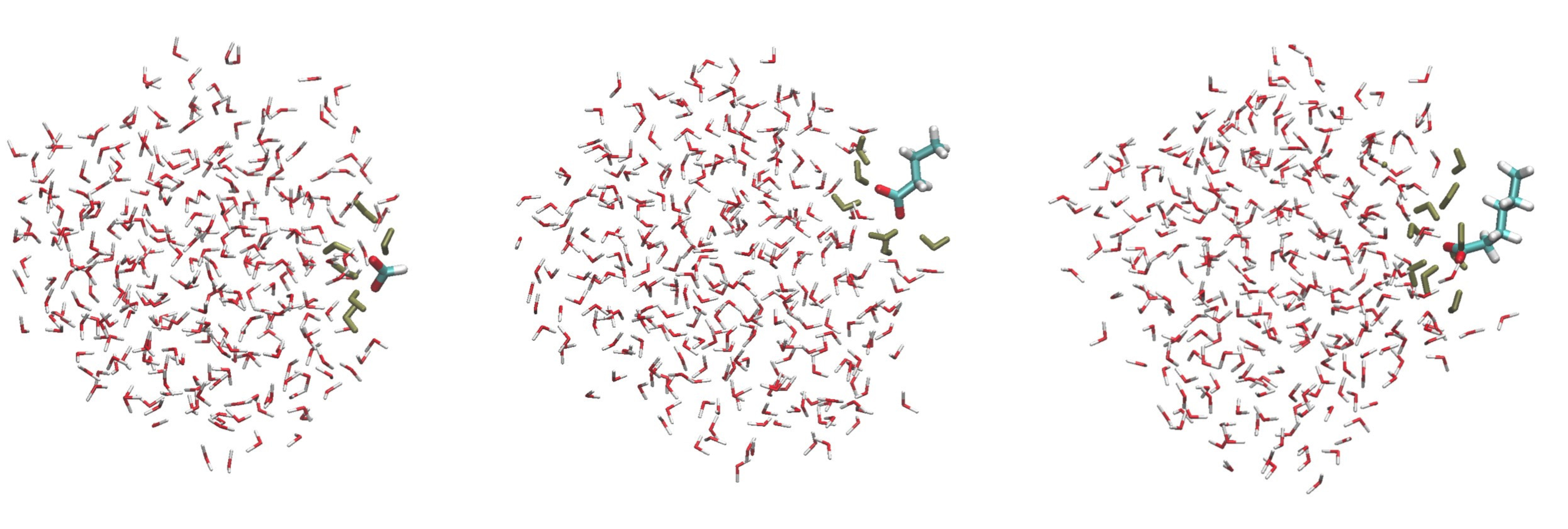
Using the strong hydrogen bond term $U^\mathrm{shb}$, we developed a force field able to model the hydration of the halides $\ce{F^-}$ to $\ce{As^-}$, as well as the hydration of linearly alkylated carboxylates. Regarding the halide $\ce{As^-}$ we showed its diffusion coefficient in aqueous phase at ambient conditions to be close to the $\ce{I^-}$ one, in agreement with recent experimental findings, see Ref. Inorganic Chemistry 57 (2018) 4926. Regarding linearly alkylated carboxylates, we showed their propensity for water droplet and liquid water interfaces to increase with the length of their alkyl chain. At water interfaces, the anionic head $\ce{COO^-}$ remains solvated while the alkyl chain points outside of the water system interface, see the following figure where three MD simulation snapshots of methanoate, butanoate and pentanoate carboxylates interacting with a 300 water droplet is shown
Regarding heavy cations, we developed a force field based on the energy term $U^\mathrm{tc}$ that allows to investigate the hydration process of two heavy cations, namely $\ce{Cm^{3+}}$ and $\ce{Th^{4+}}$. See Réal et al. (2010) and Réal et al. (2013).
Extrapolating bulk phase hydration enthalpies of single organic ions from droplet simulations
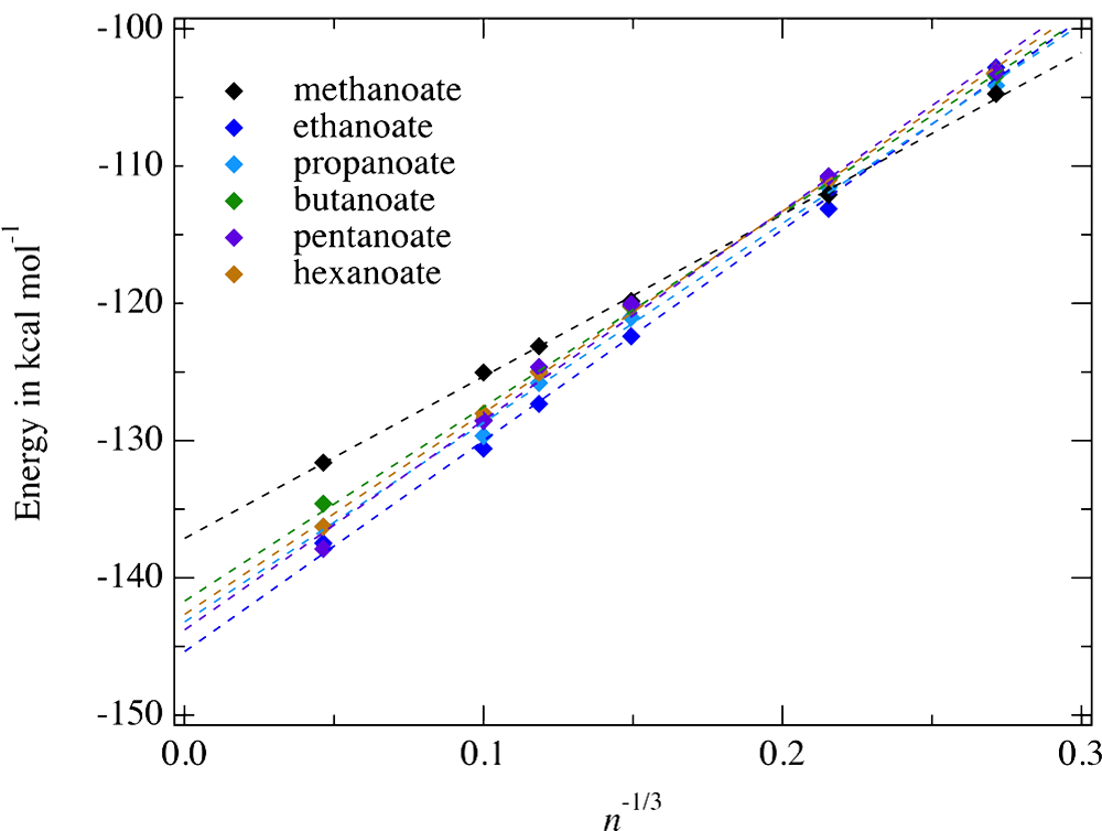
To assess the reliability of ion hydration enthalpy values computed according to that protocol, we estimate the proton hydration enthalpy from the above ion hydration enthalpy and by considering well accepted experimental data, like the enthalpy component of the ion proton affinity in gas phase, the hydration enthalpy of the neutral species (protonated or unprotonated one) corresponding to the ion, and the dissociation data corresponding to the protonation/deprotonation reaction of that ion in bulk water. For instance, the proton hydration enthalpy can be computed from data corresponding to the carboxylate $\ce{C^-}$ according to $$ \Delta H_{q \rightarrow aq} (\mathrm{H^+}) = \Delta H_{g \rightarrow aq} (\mathrm{CH}) + \Delta H_{aq,dissociation} (\mathrm{CH}) - \Delta H_{g \rightarrow aq}(\mathrm{C^-}) + \Delta H_{g,prot} (\mathrm{C^-}). $$ From methylated ammonium droplet simulations, we estimate $\Delta H_{g \rightarrow aq} (\mathrm{H^+})$ to be about 272-273 kcal mol$^{-1}$ in between the two most accepted experimental values, i.e. 271.6 and 274.9 kcal mol$^{-1}$. For carboxylates, our former droplet simulations yield a $\Delta H_{g \rightarrow aq} (\mathrm{H^+})$ value of 268 kcal mol $^{-1}$ clearly outside the latter experimental range of values. However, we identify recently a drawbacks of the water model TCPE/2013 in accurately modeling large sized anion first hydration shell structures. Remediating that drawback allows us to predict now a proton hydration enthalpy values from mono atomic halide anions (from $\ce{F^-}$ to $\ce{I^-}) $ and carboxylate $\ce{CH_3COO^-}$ droplet data in line with the above ammonium-based estimate, about 273 kcal mol$^{-1}$.
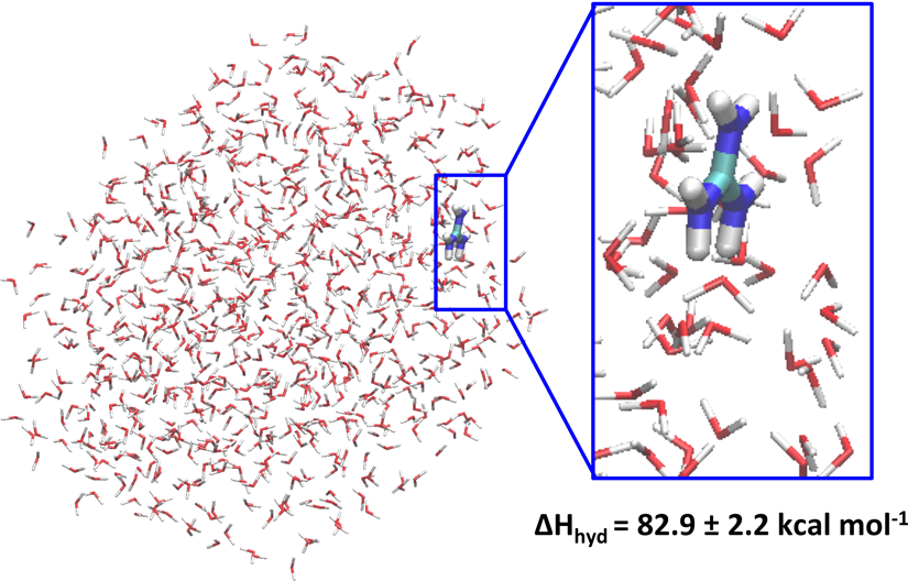
Lastly, for two ions for which experimental data are not available or are considered as puzzling, like the halide $\ce{As^-}$ and the organic cation guanidinium, our droplet-based simulation protocol yields the single ion hydration enthalpy values of 59 and 83 kcal mol$^{-1}$ for both these ions, respectively. These values are close to those computed for $\ce{I^-}$ and $\ce{NH_4^+}$, respectively. See also the following snapshot extracted from a MD simulation and showing the guanidinium ion interacting at the water droplet/air interface taken from Houriez et al. (2017).
A polarizable coarse grained approach to model the solvent water
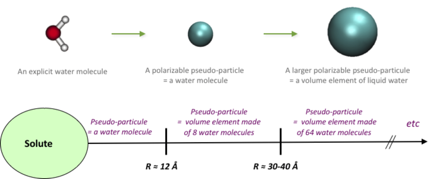
In such a pseudo particle approach, the solute/solvent and solvent/solvent interactions are truncated for large distances, the approach complexity scales as O(N). More details may be found in Masella et al. (2013). Lastly, we assign the parameters tied to particle/particle interactions to reproduce the hydrophobic effects as defined by the Lum-Chandler-Weeks theory (see Masella et al. 2011). Combined with the TCPE force fields to handle intra solute interactions, our CG approach has been shown to accurately model ion pairs in water and the solvent effect on the conformation of small peptides. We have also shown its ability to efficiently model hydrated proteins
The Multiple Time Steps approach r-RESPAp
We show the efficiency of that MTS scheme to depend on the number of iterations to converge to 'full' dipole moments each $m$ molecular dynamics iterations. However, using basic predictors, we are able to converge these dipoles within less than 8 iterations. That allows speed up factor larger than 3 when simulating a bulk phase system comprising about 3 000 atoms, using periodic boundary conditions and standard Particle Mesh Ewald sum techniques, as compared to converge the full dipole set each MD iteration. More details may be found in (Masella 2006).
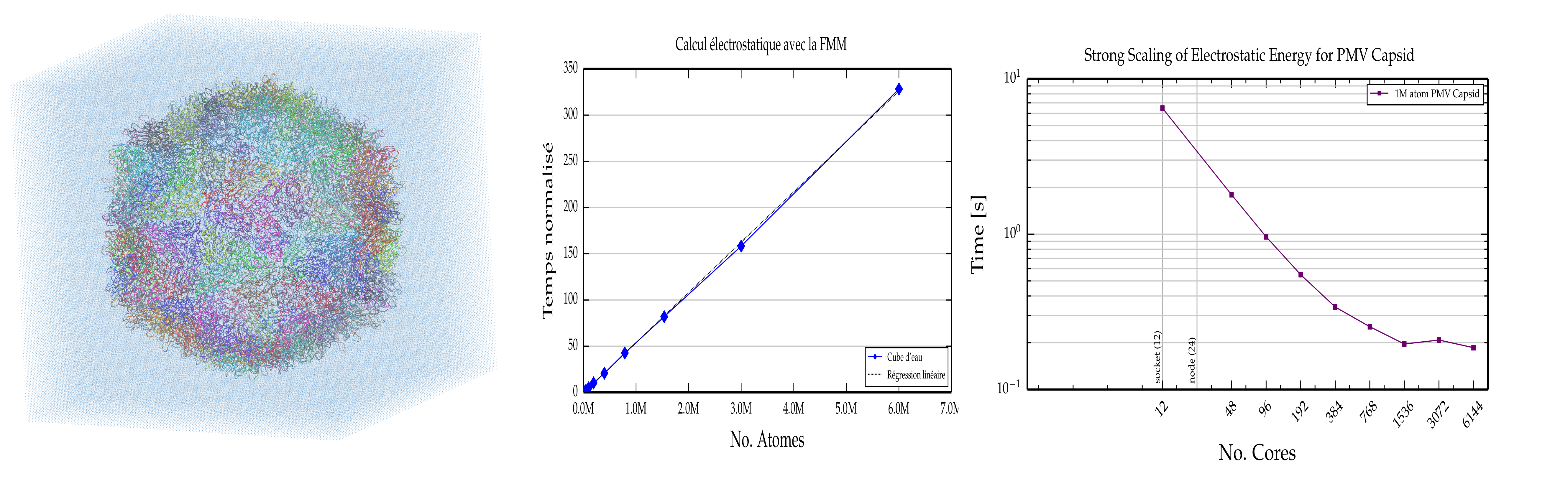
A Fast Multipole Method to model non-periodic systems
POLARIS(MD) efficiency
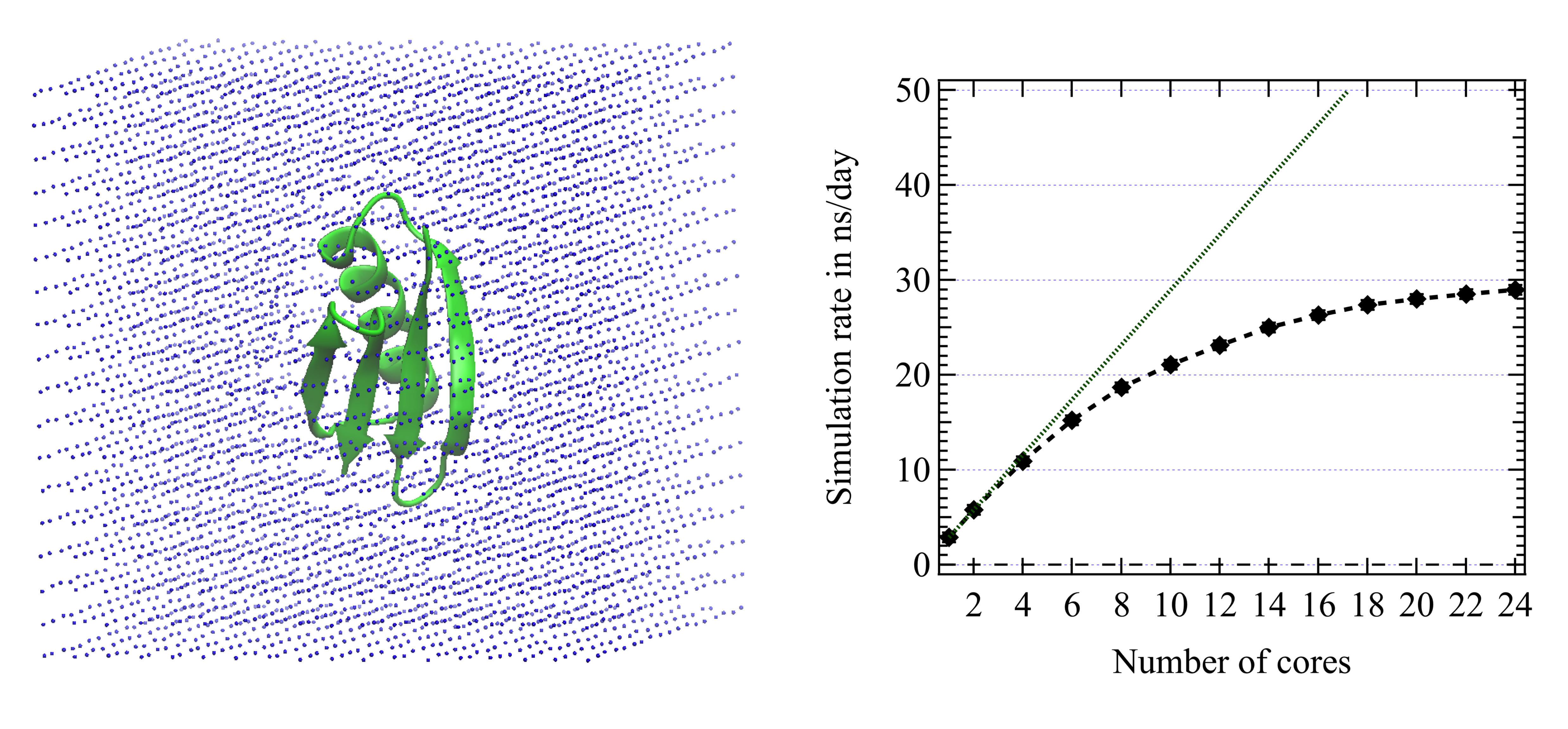
Here the system simulated is the protein 1PGB (855 atoms) embedded in a first level coarse grained solvent cubic box (Masella et al. 2013) and comprising about 5500 pseudo-particles (see below). The box dimension is about 55 Angstrom. The simulation is performed in the NVT ensemble with the temperature monitored by the GGMT thermostat (Liu 2000). The point induced dipole moments are iteratively solved until to reach a mean dipole difference between two successive iterations smaller than 10$^{-6}$ Debye and a maximum difference for a single dipole of $15\times10^{-6}$ Debye. XH bonds and HXH bond angles are constrained using the RATTLE procedure (the convergence criterium is 10$^{-6}$). We use the standard Verlet scheme to integrate the Newtonian equations of motion (and not the Multiple Time Step scheme described above). The integration time step is 2 fs.
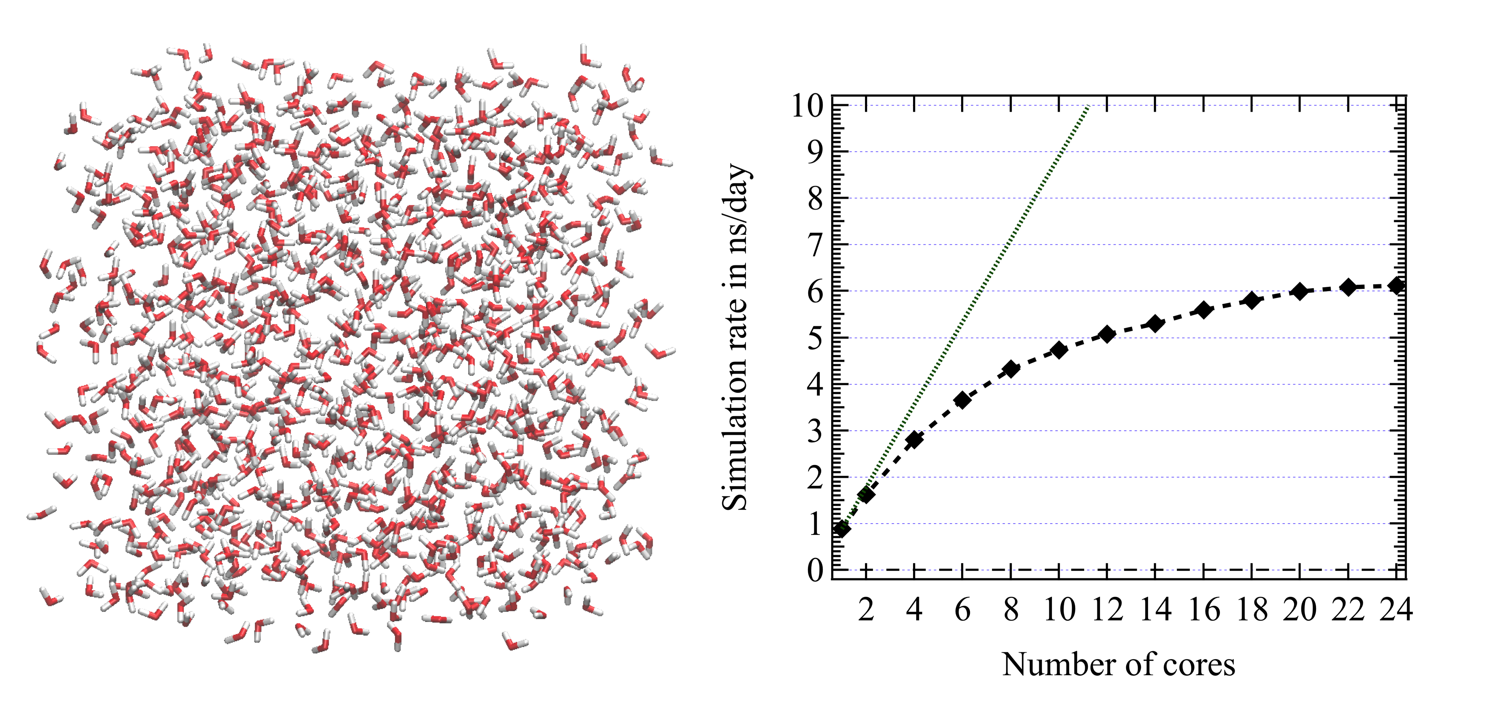
Here the system simulated is cubic box comprising 1 000 water molecules using the force field TCPE/2013 (Réal 2013). The simulation is performed in the NPT ensemble using the Nose-Hoover themostat/barostat (Martyna et al. 1996). With use infinite periodic conditions and the "full" Coulombic and polarization atomic forces are computed using the SPME approach (Toukmaji 2000) using a grid size of 1 Angstrom, 8th order interpolation spline polynomials, and a direct sum precision of 10$^{-6}$. The Fast Fourier Transform are computed using the FFTW 3 library. No surface term is considered here. The point induced dipole moments are iteratively solved until to reach a mean dipole difference between two successive iterations smaller than 10$^{-6}$ Debye and a maximum difference for a single dipole of $20\times10^{-6}$ Debye. OH bonds and HOH bond angles are constrained using the RATTLE procedure (the convergence criterium is 10$^{-6}$ Angstroms). We use the r-RESPAp scheme to integrate the Newtonian equations of motion with a short range time step of 1 fs and long range time step of 5 fs.
Regarding the FFM approach implemented in POLARIS(MD), the following right plot shows the strong scaling of a single electrostatic calculation made with FMM (from computations performed on the Hazelhen supercomputing system, Stuttgard, Germany), using the Satellite Panicum Mosaic Virus capsid with 550,620 atoms (the capsid 3D structure solvated in a solvent box comprising about 1.8 M water pseudo-particles is shown on the following left figure). The central plot shows the linear scaling of the FFM energy function computational time as a function of the atomic size of water droplets up to a 2 M water droplet..